For any service company that bills on a recurring basis, a key variable is the rate of churn. Harvard Business Review, March 2016

For just about any growing company in this “as-a-service” world, two of the most important metrics are customer churn and lifetime value. Entrepreneur, February 2016

Introduction

Customer churn occurs when customers or subscribers stop doing business with a company or service, also known as customer attrition. It is also referred as loss of clients or customers. One industry in which churn rates are particularly useful is the telecommunications industry, because most customers have multiple options from which to choose within a geographic location.

Similar concept with predicting employee turnover, we are going to predict customer churn using telecom dataset. We will introduce Logistic Regression, Decision Tree, and Random Forest. But this time, we will do all of the above in R. Let’s get started!

Data Preprocessing

The data was downloaded from IBM Sample Data Sets. Each row represents a customer, each column contains that customer’s attributes:

library(plyr)
library(corrplot)
library(ggplot2)
library(gridExtra)
library(ggthemes)
library(caret)
library(MASS)
library(randomForest)
library(party)churn <- read.csv('Telco-Customer-Churn.csv')
str(churn)

• customerID
• gender (female, male)
• SeniorCitizen (Whether the customer is a senior citizen or not (1, 0))
• Partner (Whether the customer has a partner or not (Yes, No))
• Dependents (Whether the customer has dependents or not (Yes, No))
• tenure (Number of months the customer has stayed with the company)
• PhoneService (Whether the customer has a phone service or not (Yes, No))
• MultipleLines (Whether the customer has multiple lines r not (Yes, No, No phone service)
• InternetService (Customer’s internet service provider (DSL, Fiber optic, No)
• OnlineSecurity (Whether the customer has online security or not (Yes, No, No internet service)
• OnlineBackup (Whether the customer has online backup or not (Yes, No, No internet service)
• DeviceProtection (Whether the customer has device protection or not (Yes, No, No internet service)
• TechSupport (Whether the customer has tech support or not (Yes, No, No internet service)
• streamingTV (Whether the customer has streaming TV or not (Yes, No, No internet service)
• streamingMovies (Whether the customer has streaming movies or not (Yes, No, No internet service)
• Contract (The contract term of the customer (Month-to-month, One year, Two year)
• PaperlessBilling (Whether the customer has paperless billing or not (Yes, No))
• PaymentMethod (The customer’s payment method (Electronic check, Mailed check, Bank transfer (automatic), Credit card (automatic)))
• MonthlyCharges (The amount charged to the customer monthly — numeric)
• TotalCharges (The total amount charged to the customer — numeric)
• Churn ( Whether the customer churned or not (Yes or No))

The raw data contains 7043 rows (customers) and 21 columns (features). The “Churn” column is our target.

We use sapply to check the number if missing values in each columns. We found that there are 11 missing values in “TotalCharges” columns. So, let’s remove all rows with missing values.

sapply(churn, function(x) sum(is.na(x)))

churn <- churn[complete.cases(churn), ]

Look at the variables, we can see that we have some wrangling to do.

1. We will change “No internet service” to “No” for six columns, they are: “OnlineSecurity”, “OnlineBackup”, “DeviceProtection”, “TechSupport”, “streamingTV”, “streamingMovies”.

cols_recode1 <- c(10:15)
for(i in 1:ncol(churn[,cols_recode1])) {
        churn[,cols_recode1][,i] <- as.factor(mapvalues
                                              (churn[,cols_recode1][,i], from =c("No internet service"),to=c("No")))
}

2. We will change “No phone service” to “No” for column “MultipleLines”

churn$MultipleLines <- as.factor(mapvalues(churn$MultipleLines, 
                                           from=c("No phone service"),
                                           to=c("No")))

3. Since the minimum tenure is 1 month and maximum tenure is 72 months, we can group them into five tenure groups: “0–12 Month”, “12–24 Month”, “24–48 Months”, “48–60 Month”, “> 60 Month”

min(churn$tenure); max(churn$tenure)

[1] 1

[1] 72

group_tenure <- function(tenure){
    if (tenure >= 0 & tenure <= 12){
        return('0-12 Month')
    }else if(tenure > 12 & tenure <= 24){
        return('12-24 Month')
    }else if (tenure > 24 & tenure <= 48){
        return('24-48 Month')
    }else if (tenure > 48 & tenure <=60){
        return('48-60 Month')
    }else if (tenure > 60){
        return('> 60 Month')
    }
}churn$tenure_group <- sapply(churn$tenure,group_tenure)
churn$tenure_group <- as.factor(churn$tenure_group)

4. Change the values in column “SeniorCitizen” from 0 or 1 to “No” or “Yes”.

churn$SeniorCitizen <- as.factor(mapvalues(churn$SeniorCitizen,
                                      from=c("0","1"),
                                      to=c("No", "Yes")))

5. Remove the columns we do not need for the analysis.

churn$customerID <- NULL
churn$tenure <- NULL

Exploratory data analysis and feature selection

Correlation between numeric variables

numeric.var <- sapply(churn, is.numeric)
corr.matrix <- cor(churn[,numeric.var])
corrplot(corr.matrix, main="\n\nCorrelation Plot for Numerical Variables", method="number")

The Monthly Charges and Total Charges are correlated. So one of them will be removed from the model. We remove Total Charges.

churn$TotalCharges <- NULL

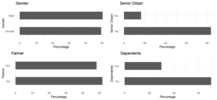
Bar plots of categorical variables

p1 <- ggplot(churn, aes(x=gender)) + ggtitle("Gender") + xlab("Gender") +
  geom_bar(aes(y = 100*(..count..)/sum(..count..)), width = 0.5) + ylab("Percentage") + coord_flip() + theme_minimal()
p2 <- ggplot(churn, aes(x=SeniorCitizen)) + ggtitle("Senior Citizen") + xlab("Senior Citizen") + 
  geom_bar(aes(y = 100*(..count..)/sum(..count..)), width = 0.5) + ylab("Percentage") + coord_flip() + theme_minimal()
p3 <- ggplot(churn, aes(x=Partner)) + ggtitle("Partner") + xlab("Partner") + 
  geom_bar(aes(y = 100*(..count..)/sum(..count..)), width = 0.5) + ylab("Percentage") + coord_flip() + theme_minimal()
p4 <- ggplot(churn, aes(x=Dependents)) + ggtitle("Dependents") + xlab("Dependents") +
  geom_bar(aes(y = 100*(..count..)/sum(..count..)), width = 0.5) + ylab("Percentage") + coord_flip() + theme_minimal()
grid.arrange(p1, p2, p3, p4, ncol=2)

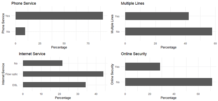
p5 <- ggplot(churn, aes(x=PhoneService)) + ggtitle("Phone Service") + xlab("Phone Service") +
  geom_bar(aes(y = 100*(..count..)/sum(..count..)), width = 0.5) + ylab("Percentage") + coord_flip() + theme_minimal()
p6 <- ggplot(churn, aes(x=MultipleLines)) + ggtitle("Multiple Lines") + xlab("Multiple Lines") + 
  geom_bar(aes(y = 100*(..count..)/sum(..count..)), width = 0.5) + ylab("Percentage") + coord_flip() + theme_minimal()
p7 <- ggplot(churn, aes(x=InternetService)) + ggtitle("Internet Service") + xlab("Internet Service") + 
  geom_bar(aes(y = 100*(..count..)/sum(..count..)), width = 0.5) + ylab("Percentage") + coord_flip() + theme_minimal()
p8 <- ggplot(churn, aes(x=OnlineSecurity)) + ggtitle("Online Security") + xlab("Online Security") +
  geom_bar(aes(y = 100*(..count..)/sum(..count..)), width = 0.5) + ylab("Percentage") + coord_flip() + theme_minimal()
grid.arrange(p5, p6, p7, p8, ncol=2)

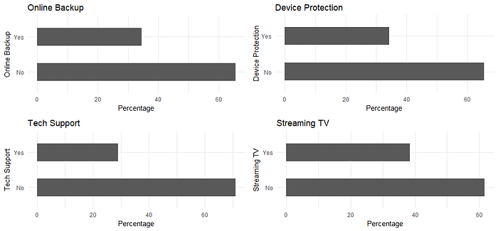
p9 <- ggplot(churn, aes(x=OnlineBackup)) + ggtitle("Online Backup") + xlab("Online Backup") +
  geom_bar(aes(y = 100*(..count..)/sum(..count..)), width = 0.5) + ylab("Percentage") + coord_flip() + theme_minimal()
p10 <- ggplot(churn, aes(x=DeviceProtection)) + ggtitle("Device Protection") + xlab("Device Protection") + 
  geom_bar(aes(y = 100*(..count..)/sum(..count..)), width = 0.5) + ylab("Percentage") + coord_flip() + theme_minimal()
p11 <- ggplot(churn, aes(x=TechSupport)) + ggtitle("Tech Support") + xlab("Tech Support") + 
  geom_bar(aes(y = 100*(..count..)/sum(..count..)), width = 0.5) + ylab("Percentage") + coord_flip() + theme_minimal()
p12 <- ggplot(churn, aes(x=StreamingTV)) + ggtitle("Streaming TV") + xlab("Streaming TV") +
  geom_bar(aes(y = 100*(..count..)/sum(..count..)), width = 0.5) + ylab("Percentage") + coord_flip() + theme_minimal()
grid.arrange(p9, p10, p11, p12, ncol=2)

p13 <- ggplot(churn, aes(x=StreamingMovies)) + ggtitle("Streaming Movies") + xlab("Streaming Movies") +
  geom_bar(aes(y = 100*(..count..)/sum(..count..)), width = 0.5) + ylab("Percentage") + coord_flip() + theme_minimal()
p14 <- ggplot(churn, aes(x=Contract)) + ggtitle("Contract") + xlab("Contract") + 
  geom_bar(aes(y = 100*(..count..)/sum(..count..)), width = 0.5) + ylab("Percentage") + coord_flip() + theme_minimal()
p15 <- ggplot(churn, aes(x=PaperlessBilling)) + ggtitle("Paperless Billing") + xlab("Paperless Billing") + 
  geom_bar(aes(y = 100*(..count..)/sum(..count..)), width = 0.5) + ylab("Percentage") + coord_flip() + theme_minimal()
p16 <- ggplot(churn, aes(x=PaymentMethod)) + ggtitle("Payment Method") + xlab("Payment Method") +
  geom_bar(aes(y = 100*(..count..)/sum(..count..)), width = 0.5) + ylab("Percentage") + coord_flip() + theme_minimal()
p17 <- ggplot(churn, aes(x=tenure_group)) + ggtitle("Tenure Group") + xlab("Tenure Group") +
  geom_bar(aes(y = 100*(..count..)/sum(..count..)), width = 0.5) + ylab("Percentage") + coord_flip() + theme_minimal()
grid.arrange(p13, p14, p15, p16, p17, ncol=2)

All of the categorical variables seem to have a reasonably broad distribution, therefore, all of them will be kept for the further analysis.

Logistic Regression

First, we split the data into training and testing sets:

intrain<- createDataPartition(churn$Churn,p=0.7,list=FALSE)
set.seed(2017)
training<- churn[intrain,]
testing<- churn[-intrain,]

Confirm the splitting is correct:

dim(training); dim(testing)

[1] 4924 19

[1] 2108 19

Fitting the Logistic Regression Model:

LogModel <- glm(Churn ~ .,family=binomial(link="logit"),data=training)
print(summary(LogModel))

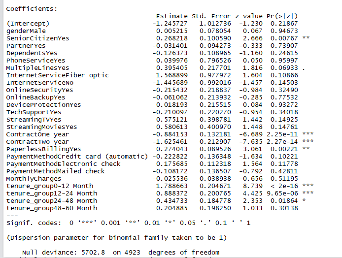
Feature Analysis:

The top three most-relevant features include Contract, tenure_group and PaperlessBilling.

anova(LogModel, test="Chisq")

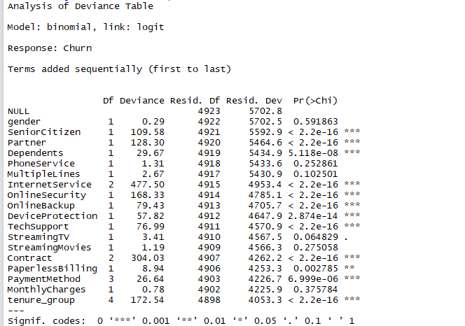
Analyzing the deviance table we can see the drop in deviance when adding each variable one at a time. Adding InternetService, Contract and tenure_group significantly reduces the residual deviance. The other variables such as PaymentMethod and Dependents seem to improve the model less even though they all have low p-values.

Assessing the predictive ability of the Logistic Regression model

testing$Churn <- as.character(testing$Churn)
testing$Churn[testing$Churn=="No"] <- "0"
testing$Churn[testing$Churn=="Yes"] <- "1"
fitted.results <- predict(LogModel,newdata=testing,type='response')
fitted.results <- ifelse(fitted.results > 0.5,1,0)
misClasificError <- mean(fitted.results != testing$Churn)
print(paste('Logistic Regression Accuracy',1-misClasificError))

[1] Logistic Regression Accuracy 0.789373814041746

Logistic Regression Confusion Matrix

print("Confusion Matrix for Logistic Regression"); table(testing$Churn, fitted.results > 0.5)

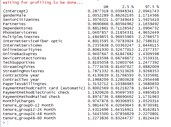
Odds Ratio

One of the interesting performance measurements in logistic regression is Odds Ratio.Basically, Odds ratio is what the odds of an event is happening.

library(MASS)
exp(cbind(OR=coef(LogModel), confint(LogModel)))

Decision Tree

Decision Tree visualization

For illustration purpose, we are going to use only three variables for plotting Decision Trees, they are “Contract”, “tenure_group” and “PaperlessBilling”.

tree <- ctree(Churn~Contract+tenure_group+PaperlessBilling, training)
plot(tree)

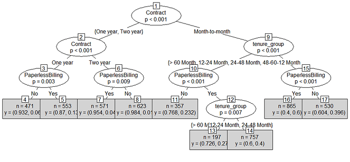
1. Out of three variables we use, Contract is the most important variable to predict customer churn or not churn.
2. If a customer in a one-year or two-year contract, no matter he (she) has PapelessBilling or not, he (she) is less likely to churn.
3. On the other hand, if a customer is in a month-to-month contract, and in the tenure group of 0–12 month, and using PaperlessBilling, then this customer is more likely to churn.

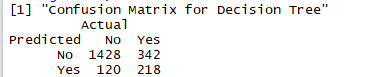
Decision Tree Confusion Matrix

We are using all the variables to product confusion matrix table and make predictions.

pred_tree <- predict(tree, testing)
print("Confusion Matrix for Decision Tree"); table(Predicted = pred_tree, Actual = testing$Churn)

Decision Tree Accuracy

p1 <- predict(tree, training)
tab1 <- table(Predicted = p1, Actual = training$Churn)
tab2 <- table(Predicted = pred_tree, Actual = testing$Churn)
print(paste('Decision Tree Accuracy',sum(diag(tab2))/sum(tab2)))

[1] Decision Tree Accuracy 0.780834914611006

The accuracy for Decision Tree has hardly improved. Let’s see if we can do better using Random Forest.

Random Forest

Random Forest Initial Model

rfModel <- randomForest(Churn ~., data = training)
print(rfModel)

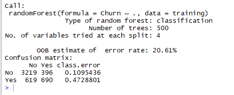
The error rate is relatively low when predicting “No”, and the error rate is much higher when predicting “Yes”.

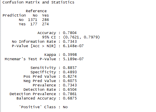
Random Forest Prediction and Confusion Matrix

pred_rf <- predict(rfModel, testing)
caret::confusionMatrix(pred_rf, testing$Churn)

Random Forest Error Rate

plot(rfModel)

We use this plot to help us determine the number of trees. As the number of trees increases, the OOB error rate decreases, and then becomes almost constant. We are not able to decrease the OOB error rate after about 100 to 200 trees.

Tune Random Forest Model

t <- tuneRF(training[, -18], training[, 18], stepFactor = 0.5, plot = TRUE, ntreeTry = 200, trace = TRUE, improve = 0.05)

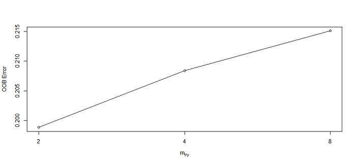
We use this plot to give us some ideas on the number of mtry to choose. OOB error rate is at the lowest when mtry is 2. Therefore, we choose mtry=2.

Fit the Random Forest Model After Tuning

rfModel_new <- randomForest(Churn ~., data = training, ntree = 200, mtry = 2, importance = TRUE, proximity = TRUE)
print(rfModel_new)

OOB error rate decreased to 20.41% from 20.61% on Figure 14.

Random Forest Predictions and Confusion Matrix After Tuning

pred_rf_new <- predict(rfModel_new, testing)
caret::confusionMatrix(pred_rf_new, testing$Churn)

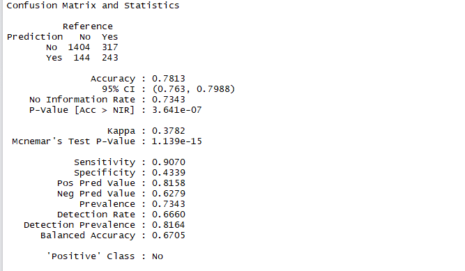
Both accuracy and sensitivity are improved, compare with Figure 15.

Random Forest Feature Importance

varImpPlot(rfModel_new, sort=T, n.var = 10, main = 'Top 10 Feature Importance')

Summary

From the above example, we can see that Logistic Regression, Decision Tree and Random Forest can be used for customer churn analysis for this particular dataset equally fine.

Throughout the analysis, I have learned several important things:

• Features such as tenure_group, Contract, PaperlessBilling, MonthlyCharges and InternetService appear to play a role in customer churn.
• There does not seem to be a relationship between gender and churn.
• Customers in a month-to-month contract, with PaperlessBilling and are within 12 months tenure, are more likely to churn; On the other hand, customers with one or two year contract, with longer than 12 months tenure, that are not using PaperlessBilling, are less likely to churn.

Source code that created this post can be found here. I would be pleased to receive feedback or questions on any of the above.